Random selection from a list in 3 steps!
- Feb 14, 2018
- 2 min read

Have you ever wanted to select items at random from a list? How did you do it? Reasons why you’d need to do random selection varies but most commonly it’s because you want to perform some testing or random sampling.
Example
I’ve got some sales products sample data from IBM. Just to give you an idea, there are more than 80,000 rows so it will be difficult to select by hand (or out of a hat, if you will). I want to select 100 from the sample.

STEP 1
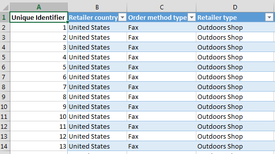
I’m going to see whether there are any unique identifiers (e.g. account number, customer ID, etc.) There doesn’t look like there’s any. I’ll add a column so that each row has a unique identifier (like a row number).

STEP 2
Using the INDEX and RANDBETWEEN formulas, I can select my sample of 100.
Excel Formula: =INDEX(array,RANDBETWEEN(bottom,top))
Formula Made Easy

Based on the photo in step 1, if I were to fill in the cell references into my Formula Made Easy table, it will look like:

Formula Applied
Putting the above references into the Excel formula, it will be:
=INDEX($A$2:$A$88476,RANDBETWEEN(2,88476))
Notice that I put $ signs between A2 and A88476 as when I drag the formulas down, I don’t want my range to change (I explain more on absolute cell referencing here).
With regards to the RANDBETWEEN component, just put in the cell number, not letter. I can see down the bottom that I’ve got my sample of 100.

The numbers will change once I click in any cell and press ENTER or continue copying / dragging the formula down. Once I’ve got my sample, I’ll highlight them, copy and paste special values (shortcut: CTRL + C to copy, CTRL + ALT + V + V + ENTER to paste special values).
STEP 3
I’ll copy my random selection (unique identifier) into a separate sheet as well as the row headers. Using INDEX-MATCH, I can get the remaining row data based on my unique identifiers. If you’re not sure how to use INDEX-MATCH, you can check out my blog post here.
The index-match formula used is:
=INDEX('WA_Sales_Products_2012-14'!B:B,MATCH(A2,'WA_Sales_Products_2012-14'!A:A,0))

Download the sample data from IBM and give it a go here.
Reference:
Sample data sourced from IBM Watson Analytics


Comments